At Skipjaq, we are interested in how applications perform as they approach the maximum sustainable load. We don’t want to completely saturate an application so it falls over, but we also don’t want to under-load the application and miss out on true performance numbers. In particular, we are interested in finding points in the load where latencies are on the precipice of moving outside acceptable limits.
In a recent conversation with the team about web application latencies, I mentioned that, as a general rule, we should expect latencies to degrade sharply once the service hits around 80% utilisation. More specifically, we should expect the wait time of the service to degrade, which will cause the latency to degrade in turn.
John D. Cook wrote a great explanation of why this is the case, but I wanted to write a slightly deeper explanation for those who have no prior experience with queuing theory.
Services as Queues
The argument for why latency degrades so badly at 80% follows directly from the results of queuing theory. We can start to understand this by first understanding how a service like a web application can be modelled using queuing theory.
For the purpose of this discussion, we’ll assume that we are interested in measuring the latency of a web application - the service - and that we are running that application on a single server. Requests arrive at the service and are processed as quickly as possible. If the service is too busy processing other requests when a new request arrives, then that request waits in the queue until the service can process it. For simplicity, we’ll assume that the queue is unbounded and that once a request is in the queue, the only way it can leave is by getting processed by the service.
The simplest queue model we can ascribe to our service is the \(M/M/1\) model. This notation is called Kendall’s notation and takes the general form \(A/S/c\), where \(A\) is the arrival process, \(S\) is the service time distribution and \(c\) is the number of servers.
Our fictional service has only one server hence \(c = 1\). The \(M\) in the model stands for Markov. The Markovian arrival process describes a Poisson process, that is a process where the time between each arrival and the next (the inter-arrival time) is exponentially-distributed with parameter \(\lambda\). The Markovian service time distribution has service times exponentially-distributed with parameter \(\mu\).
Queue Utilisation
We define service utilisation as the percentage of time the service is busy serving requests. For \(M/M/1\) queues, the utilisations is given by \(\rho = \lambda / \mu\). The queue is only stable when \(\rho < 1\). This makes intuitive sense; if there are more arrivals than can be processed by the server, then the queue will grow indefinitely.
Calculating Latency
Little’s Law is one of the most interesting results from queuing theory. Put simply it states that the average number of customers in a stable system (\(L\)) is equal to the arrival rate (\(\lambda\)) multiplied by the average time a customer spends in the system (\(W\)):
\[L = \lambda W\]The average time a customer spends in the system is equivalent to the average latency a customer will see. This value is a combination of the average service time and the average time spent waiting in the queue. Intuitively we should realise that, in a running system, the average service time is broadly fixed and that latency variations typically stem from variations in the wait time.
Since we are interested in calculating latency and not the average number of customers in the system, we can rearrange Little’s Law to put the latency (\(W\)) on the left-hand side:
\[W = \frac{L}{\lambda}\]So now, if we know the average number of customers in the system, we can calculate the wait time. The mean number of customers in an \(M/M/1\) queue is given by:
\[\frac{\rho}{1 - \rho}\]Deriving this equation from first principles is beyond the scope of this blog, but it follows from the steady-state probabilities of the Markov chain describing the process. You can find a good description of the maths behind this here.
Reminding ourselves that \(\rho = \lambda / \mu\):
\[W = \frac{\frac{\rho}{1 - \rho}}{\lambda} = \frac{\rho}{\lambda (1 - \rho)} = \frac{1 / \mu}{1 - \rho} = \frac{1}{\mu - \lambda}\]So now we have a simple formula that relates latency to the arrival rate and the service rate, but what we really want is a formula relating utilisation to latency. To do this, recognise that \(\lambda = \rho \mu\):
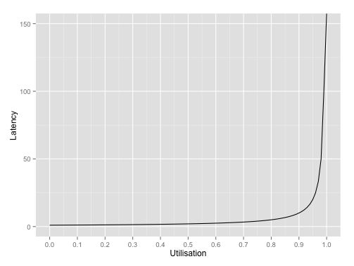
\[W = \frac{1}{\mu - \lambda} = \frac{1}{\mu - \rho \mu} = \frac{1}{\mu (1 - \rho)}\]As discussed, we can assume that \(\mu\) is constant for a running system and that the main contribution to changes in service utilisation will come from changes in the arrival rate. Thus the latency is proportional to \(1/(1 - \rho)\). If we plot this, we can see a sharp uptick in latency when utilisation hits around 80% after which the latency tends towards infinity as the utilisation tends towards to 100%.
Conclusion
Once service utilisation exceeds 80%, latencies suffer dreadfully. To avoid being surprised by disastrous latencies in production systems, it’s important to monitor utilisation and take action as it approaches the 80% danger zone.
When testing system performance, loading a system much beyond the 80% utilisation mark will likely result in latencies that are wildly unacceptable. Load that system at close to 100% and you should expect to wait quite some time to see your tests complete!