A few questions seem to come up again and again from the people who’ve been reading my posts on queue theory. Perhaps, the most common question is: “How do I model multi-server applications using queues?”. This in an excellent question since most of us will be running production systems with more than one server, be that multiple collaborating services or just a simple load-balanced service that has a few servers sharing the same incoming queue of customers.
In this post, I want to address the simplest model for multiple servers: the \(M/M/c\) queue. Like the \(M/M/1\) queue I described in an earlier post, the \(M/M/c\) queue has inter-arrival times exponentially-distributed with rate \(\lambda\), and service rate exponentially-distributed with rate \(\mu\). The difference, which should be obvious, is that rather than having just one server, we can have any positive number.
The measure of traffic intensity for \(M/M/1\) and \(M/M/c\) queues is \(\rho = \lambda / \mu\). For \(M/M/1\) queues \(\rho\) is also the measure of utilisation, but for \(M/M/c\) queues we have utilisation \(a = \rho / c\). The stability condition for \(M/M/c\) queues is \(a = \rho / c < 1\).
What to model?
One of the most important questions we can answer is: what should be modelled as a multi-server queue? One reader asked whether a multi-threaded server is best modelled using an \(M/M/c\) queue with \(c\) equal to the number of threads. This is a tough question, but to answer we should consider the requirement that, for an \(M/M/c\) queue, each of the servers must be indendent.
If we are modelling a coarse-grained service like a web server, then I think there’s enough interference between the threads to model each server process as an \(M/M/1\) queue rather than as an \(M/M/c\) process. Indeed, we might even go further and model each distinct machine as an \(M/M/1\) queue, and only use an \(M/M/c\) queue to model multiple machines serving the same stream of customers.
If we were modelling a low-level component like a thread scheduler, then we would likely use an \(M/M/c\) queue, with \(c\) equal to the number of CPUs, but at the coarse granularity of a web server, we can safely ignore the number of CPUs and threads and use an \(M/M/1\) queue.
Steady-State Probabilities
We’ll calculate the average latency of \(M/M/c\) queues from the steady-state probabilities. As I did in the previous entries, I’m not going to discuss the derivation of these probablities (although I promise to do this in an upcoming post). Remember that the steady-state probabilities \(p_{n}\) tell us the probability of there being \(n\) customers in the system. We’ll start with \(p_{0}\):
\[p_{0} = \Bigg(\sum_{n=0}^{c-1}\frac{\rho^{n}}{n!}+\Big(\frac{\rho^{c}}{c!}\Big)\Big(\frac{1}{1 - a}\Big)\Bigg)^{-1}\]For \(n \geq 1\), we must account for two scenarios: when the number of customers is less than the number of servers (\(n < c\)), and when the number of customers is greater than or equal to the number of servers (\(n \geq c\)):
\[p_{n} = \begin{cases} p_{0} \frac{\rho^{n}}{n!} & n < c \\ p_{0} \frac{a^{n}c^{c}}{c!} & n \geq c \\ \end{cases}\]Probability of Waiting
Since we have Poisson arrivals, we can calculate the probability that a customer has to wait, by summing \(p_{n}\) starting at \(c\) and proceeding to \(\infty\): \(p_{queue} = \sum_{n=c}^{\infty}p_{n}\). The expanded form of this is called Erlang’s C Formula:
\[C(c, \rho) = \frac{\frac{\rho^c}{c!}\frac{c}{c - \rho}}{\sum_{n=0}^{c-1}\frac{\rho^{n}}{n!} + \frac{\rho^{c}c}{c!(c - \rho)}}\]If we plot this function for different values of \(c\), we can easily see how adding more servers to our system reduces the likelihood a customer will have to wait:
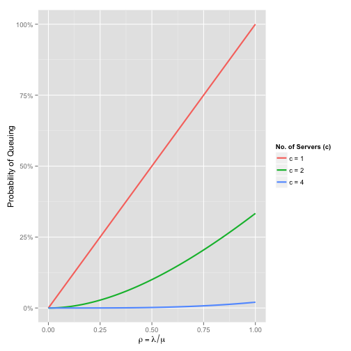
By the time we have four servers, the chance of waiting is barely noticeable, even when \(\rho = 1\).
Multi-Server Wait Times
The average time spent waiting in the queue \(W_q\) is:
\[W_q = \frac{1}{\mu(c - \rho) \cdot C(c,\rho)}\]From this we get the average latency \(W\) quite easily:
\[W = \frac{1}{\mu} + W_q\]If we plot average latency for various values of \(c\), we see how adding more servers is an effective way of reducing latency
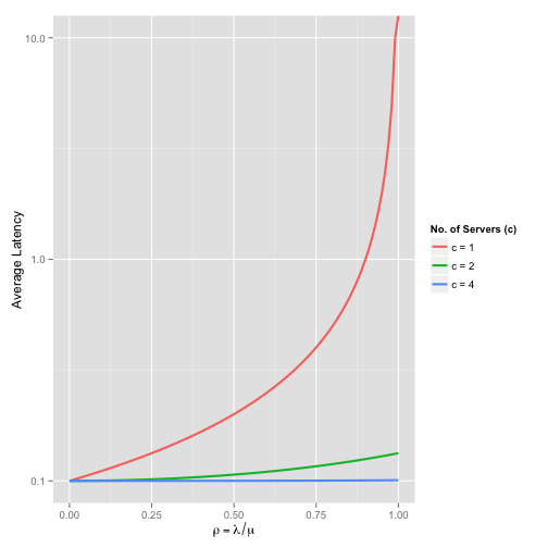
Take note of the log scale on the y-axis. At \(\rho = 1\), the \(M/M/1\) queue is at 100% utilisation and latency is tending towards \(\infty\). The extra capacity with \(c=2\) and \(c=4\) is directly reflected in the significantly smaller latencies.
Faster Servers or More Servers?
When deploying an application, it’s interesting to consider whether a smaller number of faster servers is better than a larger number of slower servers. Ignoring any discussion of reliability, we can compare the latency of different \(M/M/c\) queues to help us pick a configuration.
The plot below compares two queue models, one with \(\mu = 5\) and \(c = 3\) and the other with \(\mu = 10\) and \(c = 2\).
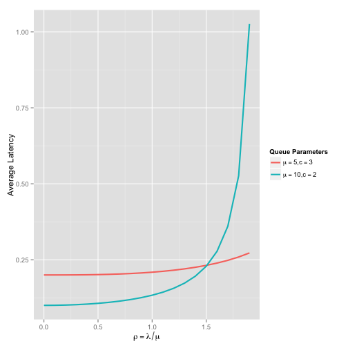
As you might expect, the queue with the lowest service rate has a higher baseline latency. However, because there are more servers in that queue, the latency as \(\rho\) increases remains steady. Recall the stability condition \(a = \lambda / (c \mu) < 1\), and it should be apparent that more servers will result in longer periods latency stability when \(\lambda > \mu\).
To see more configurations in action, I’ve created a small simulator that you can use to compare two different queue models.
Limitations of the \(M/M/c\) model
The \(M/M/c\) model is a reasonable way to model systems with multiple servers, but it has some limitations. Since the service rate \(\mu\) is a global parameter, it is not possible to model systems that have different service rates per server. In a cloud scenario you might have a set of core servers - all with the same service rate - running all the time. During periods of heavy load, you might scale up with some additional resources, but these may well have a different service rate, especially if your base servers are especially beefy.
Another limitation with the \(M/M/c\) model is that it doesn’t account for the overhead of splitting incoming traffic between the servers. In a web environment, the individual servers receive their load from some load-balancing infrastructure. The load balancer will also have a service rate describing how fast it can do its work.
In my next post, I’ll discuss addressing these weaknesses using queue networks. As the name implies, queue networks describe how individual queues are composed into collaborating networks. A web application running on two servers is described as a queue network with three nodes: one for the load balancer, and one for each of the servers.